


russtedrake PRO
Roboticist at MIT and TRI
Russ Tedrake
UCSD Contextual Robotics Seminar
May 12, 2022
Slides available live at https://slides.com/d/lwXONT0/live
or later at https://slides.com/russtedrake/2022-ucsd
Shortest Paths in Graphs of Convex Sets.
Tobia Marcucci, Jack Umenberger, Pablo Parrilo, Russ Tedrake.
Available at: https://arxiv.org/abs/2101.11565
Motion Planning around Obstacles with Convex Optimization.
Tobia Marcucci, Mark Petersen, David von Wrangel, Russ Tedrake.
Available at: https://arxiv.org/abs/2205.04422
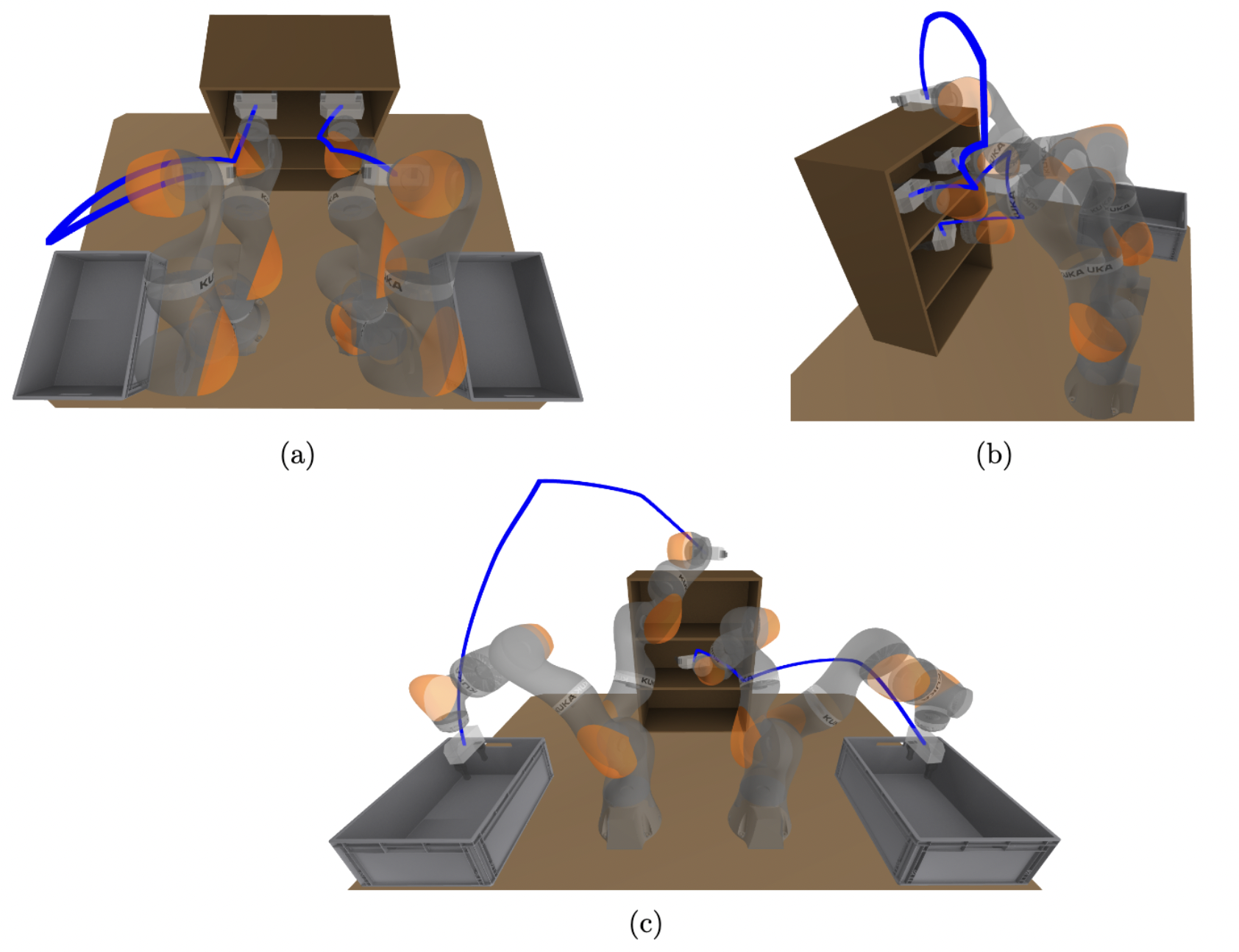
Global optimization-based planning for manipulators with dynamic constraints
image credit: James Kuffner
Trajectory optimization
Sample-based planning
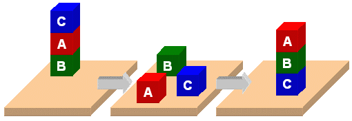
AI-style logical planning
Combinatorial optimization
start
goal
start
goal
nonconvex
fixed number of samples
Default playback at .25x
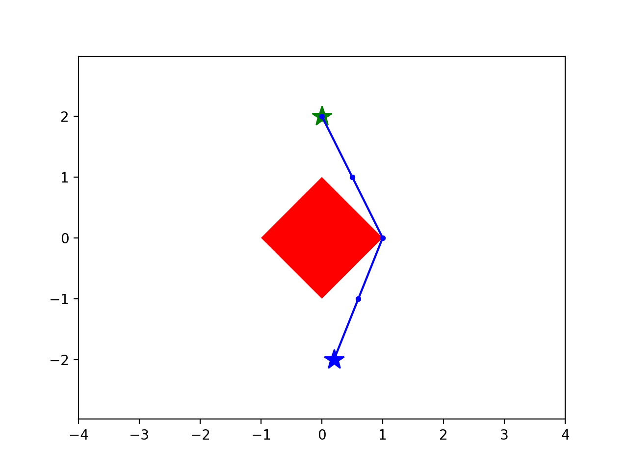
start
goal
disjunctive
constraints
Disjunctive programming leads to "loose" relaxations.
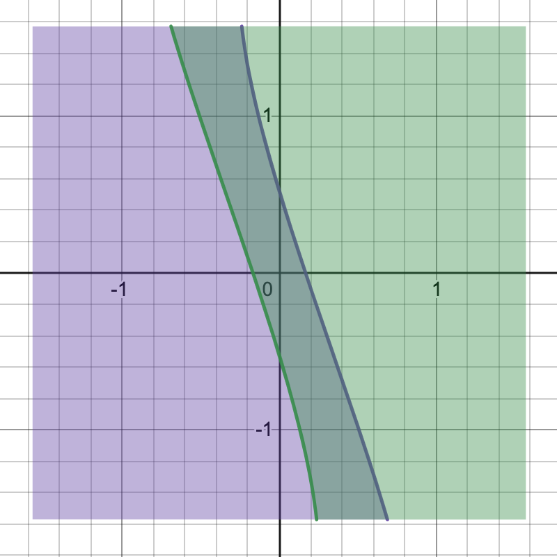
convex relaxation replaces this with:
"We know that the LP formulation of the shortest path problem is tight. Why exactly are your relaxations so loose?"
\(\varphi_{ij} = 1\) if the edge \((i,j)\) in shortest path, otherwise \(\varphi_{ij} = 0.\)
\(c_{ij} \) is the (constant) length of edge \((i,j).\)
"flow constraints"
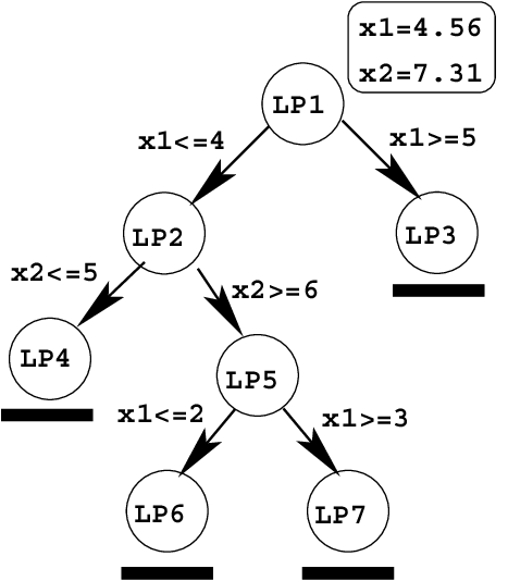
binary relaxation
path length
Classic shortest path LP
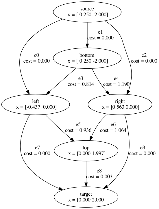
now w/ Convex Sets
start
goal
is the convex relaxation. (it's tight!)
Previous formulations were intractable; would have required \( 6.25 \times 10^6\) binaries.
| Previous best formulations | New formulation | |
|---|---|---|
| Lower Bound (from convex relaxation) |
7% of MICP | 80% of MICP |
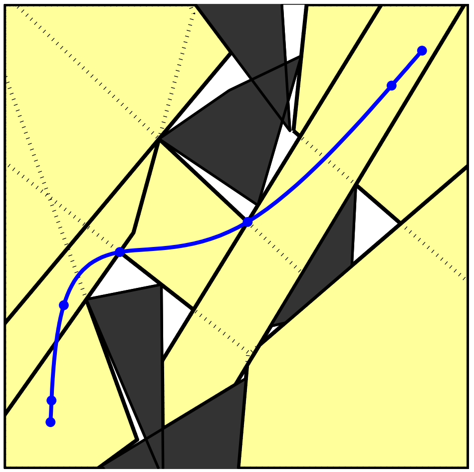
Formulating motion planning with differential constraints as a Graph of Convex Sets (GCS)
+ time-rescaling
duration
path length
path "energy"
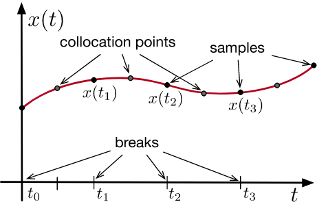
note: not just at samples
continuous derivatives
collision avoidance
velocity constraints
minimum distance
minimum time
Transcription to a mixed-integer convex program, but with a very tight convex relaxation.
IRIS (Fast approximate convex segmentation). Deits and Tedrake, 2014
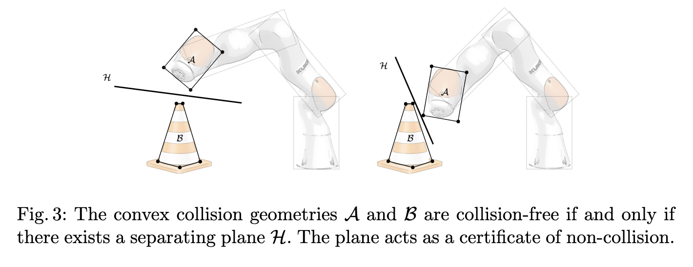
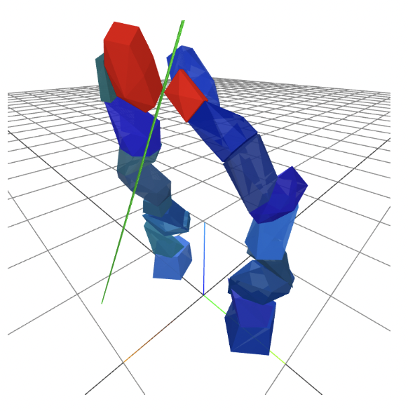
The separating plane (green) is the non-collision certificate between the two highlighted polytopic collision geometries (red), with a distance of 7.3mm.
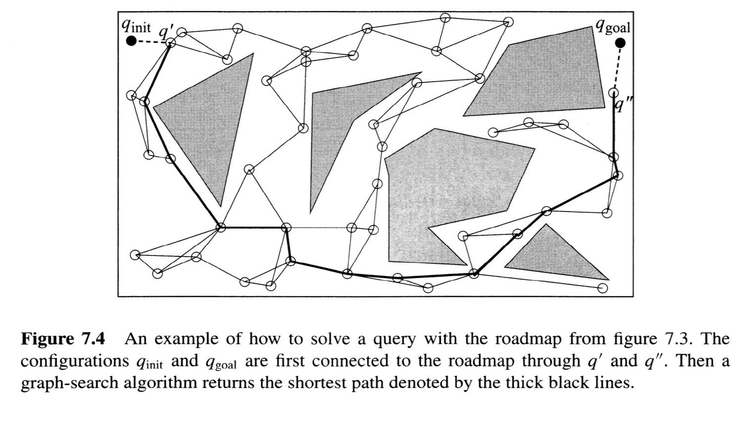
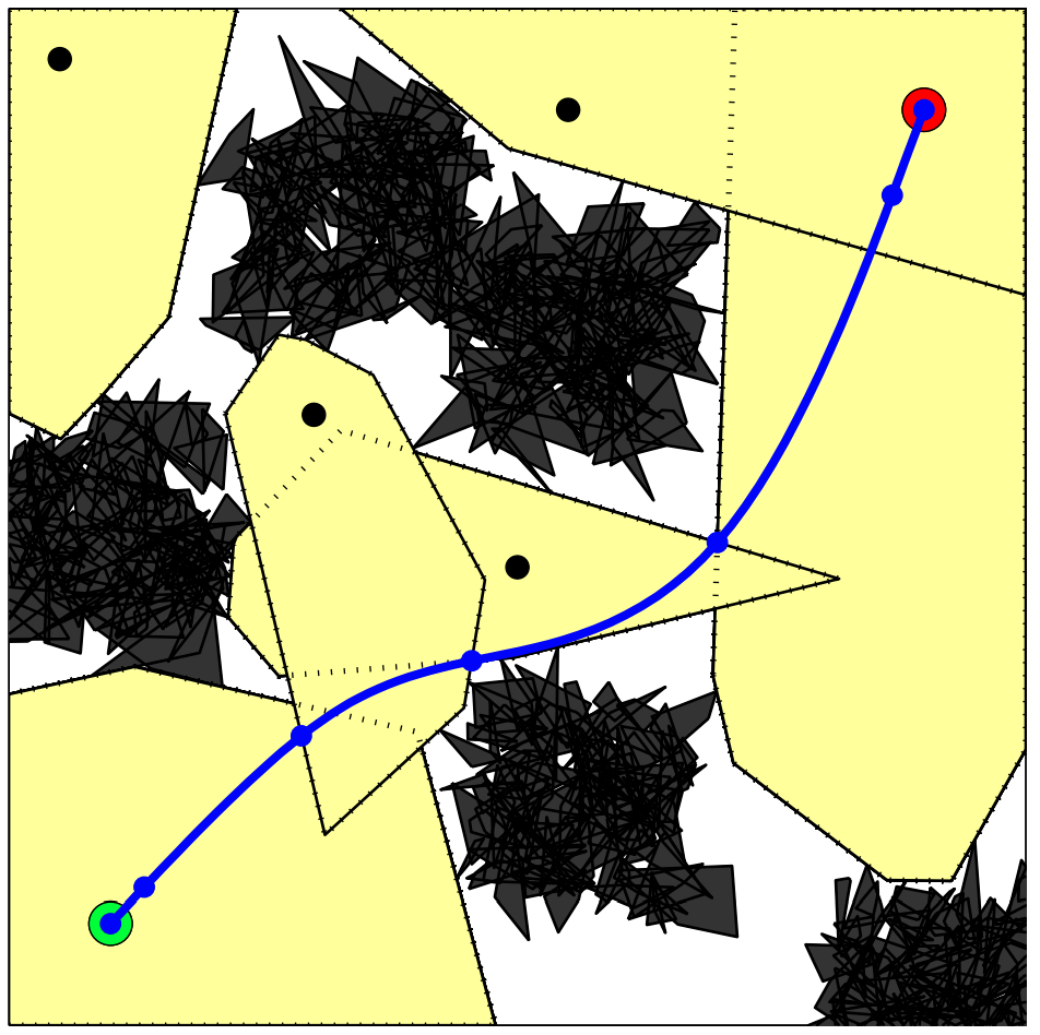
The Probabilistic Roadmap (PRM)
from Choset, Howie M., et al. Principles of robot motion: theory, algorithms, and implementation. MIT press, 2005.
Graph of Convex Sets (GCS)
PRM
PRM w/ short-cutting
Preprocessor now makes easy optimizations fast!
Note: Path length is no longer predetermined
I've focused today on Graphs of convex sets (GCS) for motion planning
GCS is a more general modeling framework
This is version 0.1 of a new framework.
There is much more to do, for example:
Give it a try:
pip install drake
sudo apt install drakeTrajectory optimization
Sample-based planning
AI-style logical planning
Combinatorial optimization
http://manipulation.mit.edu
http://underactuated.mit.edu
Shortest Paths in Graphs of Convex Sets.
Tobia Marcucci, Jack Umenberger, Pablo Parrilo, Russ Tedrake.
Available at: https://arxiv.org/abs/2101.11565
Motion Planning around Obstacles with Convex Optimization.
Tobia Marcucci, Mark Petersen, David von Wrangel, Russ Tedrake.
Available at: https://arxiv.org/abs/2205.04422
By russtedrake
Talk at UCSD, May 12, 2022


